4.5. Processing details

This section describes in details the processing workflow for the altimeter data in CCI Sea State version 4, as illustrated in figure Fig. 4.4.

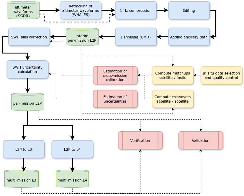
Fig. 4.4 Main steps in altimeter data processing workflow

In a nutshell:

• Significant wave height is computed from the original altimeter waveforms through the retracking step with the WHALES retracker selected by CCI Sea State expert, though for some missions the values produced by the space agencies default retracker are used.

• the full resolution SWH and sigma0 measurements are compressed to 1 Hz (one value every second) to produce a L2 product

• editing of the 1 Hz values is performed to flag bad or suspect values (and set the quality confidence variable quality_level)

• ancillary variables extracted from different sources (models and observations, climatology, land, sea ice,…) are added into the L2 product.

• bias correction of SWH is estimated for each mission to ensure consistent time series of measurements across all missions, and a corrected value added to the L2 product

• denoising is applied to the corrected SWH values using Empirical Mode Decomposition (EMD) filter and added to the L2P product as a new swh_denoised variable

• uncertainty of SWH values is estimated and added to the L2P as a new swh_uncertainty variable

• the L2P measurements are aggregated into multi-mission observation files (L3) and monthly statistics of SWH (L4) are calculated

4.5.1. SGDR input data

The table Table 4.2 summarizes the list of input altimeter data used in the processing workflow:

Table 4.2 List of SGDR input data

Mission	Version	Provider	Date
CRYOSAT-2	Version E	ESA	From 16/07/2010 to 31/12/2023
SARAL	Version F	AVISO	From 14/03/2013 to 31/12/2023
JASON-1	Version E	AVISO	From 15/01/2002 to 21/06/2013
JASON-2	Version D	AVISO	From 04/07/2008 to 01/10/2019
JASON-3	Version F	AVISO	From 17/02/2016 to 31/12/2023
TOPEX	Version F	AVISO	From 13/10/1992 to 04/10/2005
ERS-1	REAPER	ESA	From 03/08/1991 to 02/06/1996
ERS-2	REAPER	ESA	From 14/05/1995 to 02/07/2003
ENVISAT	Version 3	ESA	From 14/05/2002 to 08/04/2012
Sentinel-3A	Version 005	EUMETSAT	From 01/07/2016 to 31/12/2023
Sentinel-3B	Version 005	EUMETSAT	From 08/05/2018 to 31/12/2023
Sentinel-6A	Version F08	EUMETSAT	From 17/12/2020 to 31/12/2023

Note on TOPEX-POSEIDON

According to TOPEX version F documentation:

• From launch through repeat cycle 16, various changes to the sensors were performed. Data up to repeat cycle 16 have varying quality and should not be used for climate studies. They are ignored in CCI Dataset.

• TOPEX Side A was active from September 22, 1992 to February 10, 1999, and Side B was active from February 10, 1999 to end of mission. Users are advised to treat the data from Side A and Side B as two independent time series. No effort has been made to enforce continuity between Side A and Side B in this reprocessed data. They are separated in CCI processing.

• TOPEX Side A calibration data have a jump on April 1, 1996. This very likely causes a jump in all TOPEX altimeter geophysical measurements at this time. Users are advised to treat data from Side A1 (Launch – April 1, 1996) and Side A2 (April 1, 1996 – February 10, 1999) as two independent time series. No effort has been made to enforce continuity between Sides A1 and A2. They are separated in CCI processing.

• Sweep Calibration measurements to monitor the TOPEX point target response only started from September 8, 1998 onward for both Side A and Side B. Users are cautioned that this may cause larger errors in the reprocessed Side A data. The Sweep Calibration data available for Side A from September 8, 1998 to February 10, 1999 are not used by themselves to process the Side A data in this product. Instead, for Side A, the available Sweep Calibrations have been used to generate a model for oversampled calibrations. The nominal Cal-1 data are used with this model to process all of Side A data to generate a consistent Side A time series.

• Three 8-track tape recorders (TR A, B, C) were utilized to continuously record the 16K data stream, acquiring over 99.9% of all spacecraft and science data. However, after 5 years of excellent performance the recorders, starting with TRB, slowly started to degrade. Work arounds involving recording and playback speed restored some performance for periods. TRB was deactivated in September 2001 and TRA in October 2002. Real time acquisition through TDRSS filled much of the loss allowing approximately 90% data coverage. Finally, in October 2004 TRC failed. Real time data acquisition provided approximately 82% data coverage until the end of the mission.

4.5.2. Retracking

The retracking step calculates 20 Hz SWH measurements (40 Hz for Saral) from the altimeter waveforms available in the SGDR products (Level 1) provided by space agencies. In CCI SeaState version version 4, we have performed a complete retracking of several non-SAR altimeters with TUM’s retracker WHALES, while for others we used the full resolution SWH measurements already processed by the space agencies (see Table 4.3 for a summary). Reasons why some altimeters were not retracked with WHALES in this release include: non availability of the waveforms, non applicability of WHALES to an altimeter (e.g. SAR altimeters, lack of technical information to adapt the retracker), or postponement to a future release (Sentinel-6 LRM, ERS-1, ERS-2, …).

The Low Resolution Mode (LRM) waveforms are characterised by a rising leading edge that becomes less steep as the SWH increases, and a slowly decreasing trailing edge. The standard retracking methods are still affected by a suboptimal distribution of the residuals in the fitting process, which results in high level of noise in the estimations. WHALES is designed as a unified way to solve these problems and is based on two principles:

1. The application of a weighted fitting solution, whose weights are adapted to the SWH in order to guarantee a more uniform distribution of the residuals during the iterative fitting. This guarantees significantly more precise estimations.

2. A subwaveform strategy to focus the retracking on the portion of the signal of interest, avoiding heterogeneous backscattering in the trailing edge (partially inherited from the ALES retracker, Passaro et al., 2014). This guarantees efficiency in the coastal zone and a better representation of the oceanic scales of variability.

Moreover, a revisiting of the look-up tables used to correct for the Gaussian approximation of the Point Target Response in the Brown model ensures that the accuracy in the estimation is tailored to the new retracking solution.

References

Passaro M., Cipollini P., Vignudelli S., Quartly G., Snaith H.: ALES: A multi-mission subwaveform retracker for coastal and open ocean altimetry. Remote Sensing of Environment 145, 173-189, https://doi.org/10.1016/j.rse.2014.02.008, 2014

Table 4.3 summarized the retracker used for each mission for significant wave height, whether the retracking was performed by CCI Sea State production team (WHALES) or a third party agency:

Table 4.3 Retracker used for each mission for retrieving the significant wave height

source	period	retracker
ERS-1	07/1991 to 03/2000	REAPER (MLE3)
ERS-2	04/1995 to 07/2011	REAPER (MLE3)
Jason-1 Version E	01/2002 to 07/2013	WHALES
Jason-2 Version D	06/2008 to 10/2019	WHALES
Jason-3 Version D	09/2016 to 06/2019	WHALES
Jason-3 Version F	06/2019 to now	WHALES
Jason-3 Version T	02/2016 to 09/2016	WHALES
Topex Version F	08/1992 to 01/2006	MLE3
Envisat Version 3	03/2002 to 04/2012	WHALES
CryoSat-2 Version E	07/2010 to now	WHALES
SARAL Version F	02/2013 to now	WHALES
Sentinel-6 A Version F08	03/2020 to 12/2023	MLE4
Sentinel-3 A Version 005	02/2016 to now	MLE4
Sentinel-3 B Version 005	04/2018 to now	MLE4

For sigma0, the measurements from the original retracking performed by the agency which provided the input data (SGDR) were used, with no correction by CCI Sea State for this version. Table 4.4 summarized the retracker used for each mission for sigma0 by these agencies:

Table 4.4 Retracker used for each mission for retrieving the sigma0

source	period	retracker (per band)
ERS-1	07/1991 to 03/2000	REAPER/MLE3 (Ku)
ERS-2	04/1995 to 07/2011	REAPER/MLE3 (Ku)
Jason-1 Version E	01/2002 to 07/2013	MLE3 (Ku, C)
Jason-2 Version D	06/2008 to 10/2019	MLE3 (Ku, C)
Jason-3 Version T	02/2016 to 09/2016	MLE3 (Ku, C)
Jason-3 Version D	09/2016 to 06/2019	MLE3 (Ku, C)
Jason-3 Version F	06/2019 to now	MLE3 (Ku, C)
Topex Version F	08/1992 to 01/2006	MLE3 (Ku, C)
Envisat Version 3	03/2002 to 04/2012	MLE3 (C)
CryoSat-2 Version E	07/2010 to now	Ocean CFI/MLE4 (Ku)
SARAL Version F	02/2013 to now	MLE4 (Ka)
Sentinel-6 A Version F08	03/2020 to 12/2023	MLE3 (Ku, C)
Sentinel-3 A Version 005	02/2016 to now	MLE4 (Ku), MLE3 (C)
Sentinel-3 B Version 005	04/2018 to now	MLE4 (Ku), MLE3 (C)

4.5.3. Compression to 1 Hz

The CCI Sea State Dataset version 4 provides 1 Hz SWH measurements. These 1 Hz measurements are calculated by averaging groups of consecutive full resolution 20 Hz (18 Hz for Envisat or Topex, 40 Hz for SARAL).

The method used to average the full resolution measurements into 1 Hz values is the same for all altimeters. The groups of full resolution measurements used to calculate the 1 Hz values are exactly the same as in the source Agency’s GDR and SGDR products. Both CCI and Agency files can be compared one to one, have the same number of measurements, and the same latitude, longitude, time for each 1 Hz measurement.

For each group of valid (the measurements remaining after the editing described above) measurements, the 1 Hz SWH value is computed as the median of the remaining full resolution SWH values and copied to swh variable. Moreover, the swh_num_valid variable is computed as the number of remaining valid full resolution measurements and the swh_rms variable is computed as the root mean square of the deviation from the median, considering only valid full resolution measurements.

The same method is used to calculate 1 Hz sigma0 values from the full resolution sigma0.

The compression of the full resolution (20/40 Hz) SWH and sigma0 measurements into 1 Hz values follows these steps:

1. Full resolution (20/40 Hz) SWH and sigma0 values are flagged as land when their distance to coast is greater than 1000m, based on the Goddard Space Flight Center (GSFC) 1km resolution grid of distance to coast. They are ignored in the compression process.

2. Full resolution measurements flagged as bad by the retracker are discarded. These measurements are flagged as bad, for altimeters retracked with WHALES, when the fitting error is greater than 0.3. In Agency’s SGDR, a quality variable is usually associated with the SWH and sigma0 variables and used as a substitute here. Table 4.5 and Table 4.6 provides, respectively for SWH and sigma0, the source variable used as input for the full resolution measurements, the associated quality variable used for this editing and condition tested to discard the measurements.

3. Full resolution SWH measurements not in the -0.5 to 30 meter range are also discarded.

4. Among the remaining full resolution SWH measurements, outliers are discarded. The outlier detection scheme is based on the maximum absolute deviation (MAD) for a 3-sigma criterion, meaning:

   • only 20 Hz SWH values within [median(SWH) - 3 * MAD(SWH), median(SWH) 3 * MAD(SWH)] interval are kept

   • with: MAD(SWH) = 1.4286 * median(abs(SWH - median(SWH)))

5. The median of the remaining measurements is selected as 1 Hz value. When there were less than 6 (12 for SARAL) valid remaining measurements, the 1 Hz value is flagged as bad in the quality_level variable.

Table 4.5 selected variable for SWH in each full resolution dataset, and the corresponding quality flag variable used to discard invalid measurements

Source	SWH	SWH quality
Jason-1 Version E	swh.07	swh_WHALES_fitting_error_20hz > 0.3
Jason-2 Version D	swh.07	swh_WHALES_fitting_error_20hz > 0.3
Jason-3 Version D	swh_WHALES_20hz	swh_WHALES_fitting_error_20hz > 0.3
Jason-3 Version F	swh_WHALES_20hz	swh_WHALES_qual_20hz == 0
Jason-3 Version T	swh_WHALES_20hz	swh_WHALES_fitting_error_20hz > 0.3
Topex Version F	swh_20hz_ku	swh_used_20hz_ku == 0
Envisat Version 3	swh_WHALES_20hz	swh_WHALES_qual_20hz == 0
ERS-1 REAPER	swh_20hz	swh_used_20hz == 0
ERS-2 REAPER	swh_20hz	swh_used_20hz == 0
CryoSat-2 Version E	swh_WHALES_20hz	swh_WHALES_fitting_error_20hz > 0.3
Saral Version F	swh_WHALES_20hz	swh_WHALES_fitting_error_20hz > 0.3
Sentinel-6A Version F08	swh_ocean	swh_ocean_qual == 1
Sentinel-3A Version 005	swh_ocean_20_plrm_ku	swh_ocean_qual_20_plrm_ku == 0
Sentinel-3B Version 005	swh_ocean_20_plrm_ku	swh_ocean_qual_20_plrm_ku == 0

For the compression of the sigma0, the processing is the same. Full resolution sigma0 measurements are discarded if not in the range: [7, 30] dB (except for SARAL Ka sigma0: [-6.5, 23.]).

Important

sigma0, in C and Ku band (Ka for SARAL), are always taken from the agency’s SGDR, even when using WHALES to estimate SWH using MLE3 Ku band sigma0 when available, as summarized in Table 4.6.

Table 4.6 selected variable for sigma0 in each full resolution dataset, for each sensing band, and the corresponding quality flag variable used to discard invalid measurements

Source	Sigma0	Sigma0 quality
Jason-1 Version E	sig0_20hz_ku	sig0_used_20hz_ku == 0
	sig0_20hz_c	sig0_used_20hz_c == 0
Jason-2 Version D	sig0_20hz_ku_mle3	sig0_used_20hz_ku_mle3 == 0
	sig0_20hz_c	sig0_used_20hz_c == 0
Jason-3 Version D	sig0_20hz_ku_mle3	sig0_used_20hz_ku_mle3 == 0
	sig0_20hz_c	sig0_used_20hz_c == 0
Jason-3 Version F	ku_sig0_ocean_mle3	ku_sig0_ocean_mle3_compression_qual == 0
	c_sig0_ocean	c_sig0_ocean_compression_qual == 0
Topex Version F	sig0_20hz_ku_mle3	sig0_used_20hz_ku == 0
Envisat Version 3	sig0_ocean_20_ku	sig0_ocean_qual_20_ku == 0
ERS-1 REAPER	ocean_sig0_20hz	ocean_sig0_used_20hz
ERS-2 REAPER	ocean_sig0_20hz	ocean_sig0_used_20hz
CryoSat-2 Version E	sig0_1_20_ku
SARAL Version T	sig0_40hz	sig0_used_40hz == 0
Sentinel-6 A Version F08	ku_sig0_ocean_mle3	ku_sig0_ocean_mle3_qual != 1
	c_sig0_ocean	c_sig0_ocean_qual != 1
Sentinel-3 A Version 005	sig0_ocean_20_plrm_ku	sig0_ocean_qual_20_plrm_ku == 0
	sig0_ocean_20_c	sig0_ocean_qual_20_c == 0
Sentinel-3 B Version 005	sig0_ocean_20_plrm_ku	sig0_ocean_qual_20_plrm_ku == 0
	sig0_ocean_20_c	sig0_ocean_qual_20_c == 0

S-band sigma0 were ignored for Envisat as it was found they were systematically flagged as bad in the SGDR product.

4.5.4. Editing

The quality level of SWH measurement, provided in the quality_level variable is estimated by applying a suite of specific tests. When positive, a test will downgrade a SWH measurement (starting initially with the quality level inherited from the 1 Hz compressed data file) to a lower value, as given in the following table. The result of each applied test is summarized in the corresponding rejection_flags variable.

Table 4.7 Quality level assigned to a validity test if positive (with corresponding label in the rejection_flags variable

Validity test	Assigned quality level
sea_ice: 0 < sea ice concentration <= 10%	2
sea_ice: sea ice concentration > 10%	1
swh_validity: 0 <= SWH <= 30	1
swh_rms_outlier: SWH RMS in 1 Hz meaurement > LUT value	1
outlier_test: SWH outlier test	1

4.5.4.1. Test on SWH RMS (swh_rms_outlier)

As documented in Sepulveda et al. (2015), SWH measurements derived from radar altimeter measurements can be contaminated by the presence of land in the footprint, strong rain events, and so-called “sigma0 blooms” due to weak winds or surface slicks. According to these authors, the standard deviation of the full resolution (20Hz/40Hz) SWH values over one second (hereinafter called SWH RMS) is one of the most relevant parameter to detect erroneous values of SWH. Since the SWH RMS level strongly depends on SWH, constant threshold values are not adequate to efficiently remove SWH RMS outliers.

Therefore, Sepulveda et al. (2015) and Queffeulou (2016) proposed a methodology to set a statistical threshold on SWH RMS that depends on SWH, and which can be used a posteriori to filter out erroneous SWH measurements. Since the SWH RMS for a given narrow SWH presents a log-normal distribution, these authors proposes to estimate the upper threshold for the logarithm of SWH RMS as the sum of the mean value and thrice the standard deviation. Moreover, in order to reduce discontinuity in the SWH RMS threshold function for large SWH values, where the number of records is too low to derive robust statistics, a second-order polynomial function is fitted.

The methodology implemented to determine a SWH RMS LUT for each mission of the Sea State CCI version 4 dataset can be described as follows:

1. eight cycles of SWH and SWH RMS measurements are sampled and invalid measurements are rejected based on the land mask and SWH range quality flags;

2. for each cycle the mean and standard deviation of log(SWH RMS) are computed for SWH bins of 0.5 m width, ranging from 0 to 15 m, with a 0.05 m increment. Only bins with more than 100 values are considered;

3. upper threshold on SWH RMS are computed for each SWH bin as: \(\exp(mean(\log{}swh\_rms)+3\times std(\log{}swh\_rms))\);

4. a second-order polynomial function is fitted to the SWH RMS threshold function for SWH values comprised between 3 and 10m and is extrapolated up to SWH = 12m;

5. a look-up table (LUT) of SWH RMS thresholds is derived by combining for each cycle the SWH RMS threshold values for SWH lower than 3m and the values of the polynomial function for SWH higher than 3m; for SWH above 12 m, a constant value equal to the SWH RMS threshold at 12m is taken;

6. the final LUT is computed as the ensemble mean of the 8 cycle LUTs;

Note that the selection of the lower and upper bounds (3-10m) used to estimate the second-order polynomial function are mission specific, and is determined for each method from visual inspection of the SWH_RMS = f(SWH) function.

The cycles selected to build these LUTs, the methodology and resulting average LUTs are described in further details here.

4.5.4.2. Test on SWH outliers (outlier_test)

Above quality flags and tests are not sufficient to discard all the erroneous SWH data. Spurious measurements are still observed: some are located in the vicinity of the coast where some land can be within the altimeter footprint, or in areas of high scattering resulting in so- called sigma0 blooms (e. g. Thibaut et al. 2007). Some other individual spurious measurements (corresponding mainly to high values of SWH) are not explained. Consequently the data are filtered to eliminate these measurements.

The screening is based on the analysis of the differences between successive along track SWH measurements, using along track running windows, 100 km wide. For each measurement the along track data within 50 km each side are selected. This represents a maximun number of 15 (Envisat) to 19 (Jason) selected data. Then over this segment the 2 extreme SWH data are discarded, and the mean value (m) and standard deviation (s) are estimated over the residual data set. If the SWH value is outside the interval defined by m ± 4s, then this data is considered as erroneous and is discarded. Up to 3 iterative passes were empirically adjusted for the processing.

4.5.5. Ancillary data

The base L2 compressed files are enriched with additional external sources information.

4.5.5.1. Ancillary atmospheric model variables

Complementary ocean or atmospheric variables are taken from ECMWF ERA5 reanalysis, using spatial and temporal linear interpolation at measurement point.

Table 4.8 ERA5 atmospheric model variables added to each 1 Hz measurement in L2P

Variable	Description
tclw	Total column cloud liquid water
t2m	2 metre temperature
sst	Sea surface temperature
u10	10 metre U wind component
v10	10 metre V wind component
sp	Surface pressure

4.5.5.2. Ancillary wave model variables

Complementary sea state variables are taken from ECMWF ERA5 reanalysis (WAM model for waves) and Ifremer Wave Watch 3 hindcast run, using spatial and temporal linear interpolation at measurement point.

Table 4.9 ERA5/WAM wave model variables added to each 1 Hz measurement in L2P

Variable	Description
swh	Significant height of combined wind waves and swell
pp1d	Peak wave period
p1ps	Mean wave period based on first moment of swell
p140121	Significant wave height of first swell partition
p140122	Mean wave direction of first swell partition
mwp	Mean wave period
mwd	Mean wave direction
shww	Significant height of wind waves
mdww	Mean direction of wind waves
mpww	Mean period of wind waves

Table 4.10 Ifremer/WW3 hindcast wave model variables added to each 1 Hz measurement in L2P

Variable	Description
uwnd	10 metre U wind component
vwnd	10 metre V wind component
hs	Significant height of wind and swell waves
t02	Mean period T02
t0m1	Mean period T0m1
1/fp	Wave peak frequency
dir	Wave mean direction
skw	skewness
qkk	k-peakedness

Note

The WW3 model configuration ran for this ancillary source uses surface currents (from CMEMS) and icebergs computed from altimetry and only available from 1993. The configuration used for the years 1991-1992 is therefore different and not full consistent with the model configuration used from 1993 onward.

4.5.5.3. Ancillary sea ice concentration

Different sources are combined for sea ice concentration, as the best resolution datasets (25 km) do not cover the full CCI Sea State temporal coverage. For each source, we use the closest in time concentration map, up to three days apart in case it is missing for a given day, before switching to the next source in line.

Table 4.11 sources for sea ice concentration (SIC) CDR, by order of priority

	Variable	Temporal Coverage	Description
OSISAF-AMSR-CDR-v3p0	ice_conc	2002-2020 (ext: 2024)	AMSR Sea Ice Concentration Climate Data Record from OSI SAF (doi: 10.15770/EUM_SAF_OSI_0015)
SICCI-HR-SIC	ice_conc	1991-2020	High(er) Resolution Sea Ice Concentration Climate Data Record Version 3 from CCI Sea Ice+ (SSM/I and SSMIS) (doi: 10.5285/eade27004395466aaa006135e1b2ad1a)

4.5.5.4. Bathymetry

The bathymetry depth is taken from the 15 arc-second resolution General Bathymetric Chart of the Oceans (GEBCO), 2024 ( https://doi.org/10.5285/1c44ce99-0a0d-5f4f-e063-7086abc0ea0f) which can be found at: https://www.gebco.net/.

It is resampled on each L2P measurement location using closest neighbour.

4.5.5.5. Distance to coast

The distance to closest shoreline is taken from the gridded data set of distances from the nearest coastline available at PacIOOS (https://www.pacioos.hawaii.edu/metadata/dist2coast_1deg.html) . Negative distances represent locations over land (including land-locked bodies of water), while positive distances represent the ocean. NASA’s Ocean Biology Processing Group (OBPG) generated this data set using the Generic Mapping Tools (GMT) software package. Distances were computed with GMT using its intermediate-resolution coastline and then gridded globally at a spatial resolution of 0.04 degrees. Bilinear interpolation was then applied to increase the spatial resolution to 0.01 degrees. There is an uncertainty of up to 1 km in the computed distance at any given point.

It is resampled on each L2P measurement location using closest neighbour.

4.5.6. SWH bias correction

The bias correction method implemented for the Sea State CCI version4 dataset (hereafter CCI v4) includes two main components. The first component is the SWH cross-mission intercalibration, which aims at reducing the inter-mission bias. The second component is the SWH absolute calibration, which aims at reducing the bias between altimeter missions and in situ SWH measurement from a global wave buoy network. As implemented in the CCI v4, the method is based on three types of dataset:

• collocated SWH records from two reference missions (see definition) sharing the same orbit during their tandem phases (hereafter called tandem records);

• collocated measurements between a reference mission and a non-reference mission at their crossover locations (crossover records);

• collocated measurements between reference missions and in situ buoy SWH measurements (buoy matchup records).

Reference missions

Altimetry reference missions are satellite missions that provide high-accuracy, continuous measurements of sea surface height from a stable reference orbit, forming the backbone of global sea level monitoring. These missions include carefully coordinated tandem phases, during which a new satellite flies closely behind its predecessor to enable cross-calibration and ensure data continuity across successive missions. In this document reference altimetry missions refers to the current altimetry mission Sentinel-6 Michael Freilich and the four historical altimetry missions Topex-Poseidon, Jason-1, Jason-2, and Jason-3.

The general organization of the bias correction methodology is made of the following steps:

• the five reference missions are intercalibrated using tandem SWH records. For this purpose, Jason-3 SWH records are considered as unbiased and the four other missions are aligned to its records;

• the five intercalibrated reference missions are calibrated against in situ measurements (absolute calibration) using buoy matchups. For this purpose, it is assumed that all reference missions, once intercalibrated with each other, present similar bias patterns with respect to in situ data so that a single bias-correction function can be derived for all missions. This assumption allows to increase the number of altimeter-buoy data pairs and
  extend the validity range of the calibration ;

• the non-reference missions are intercalibrated against reference missions based on crossover records with the reference mission presenting the longest overlap with them;

4.5.6.1. Description of the correction method

Here, the correction method refers to any of the tandem-based, crossover-based or matchup-based corrections, either used for cross-mission intercalibration or absolute calibration of the reference missions. Building up on developments carried out during the first phase of the Sea State CCI project (Dodet et al. 2020), the correction method is based on data binning technique and results in Look Up Tables (LUT) that can accommodate for SWH-dependent error structures. First, the median values of the SWH residuals between uncorrected and reference dataset (see Table 1) are computed for 0.20m-SWH bin width, with a 0.05 m increment, over the full SWH range. When the number of data pairs within a given bin is too low (below 50) , a Not-a-Number (NaN) value is assigned to this particular bin. This systematically occurs at the low and high ends of the SWH distribution. In order to avoid abrupt change in the bias-corrected SWH field, the corrections are extrapolated at the low end using the first non-NaN value. For SWH above 10m, the corrections are extrapolated using the correction at SWH=10m. Fig. 4.5 gives an illustration of the method for the intercalibration step between Sentinel-6A and Jason-3 missions during their tandem phase.

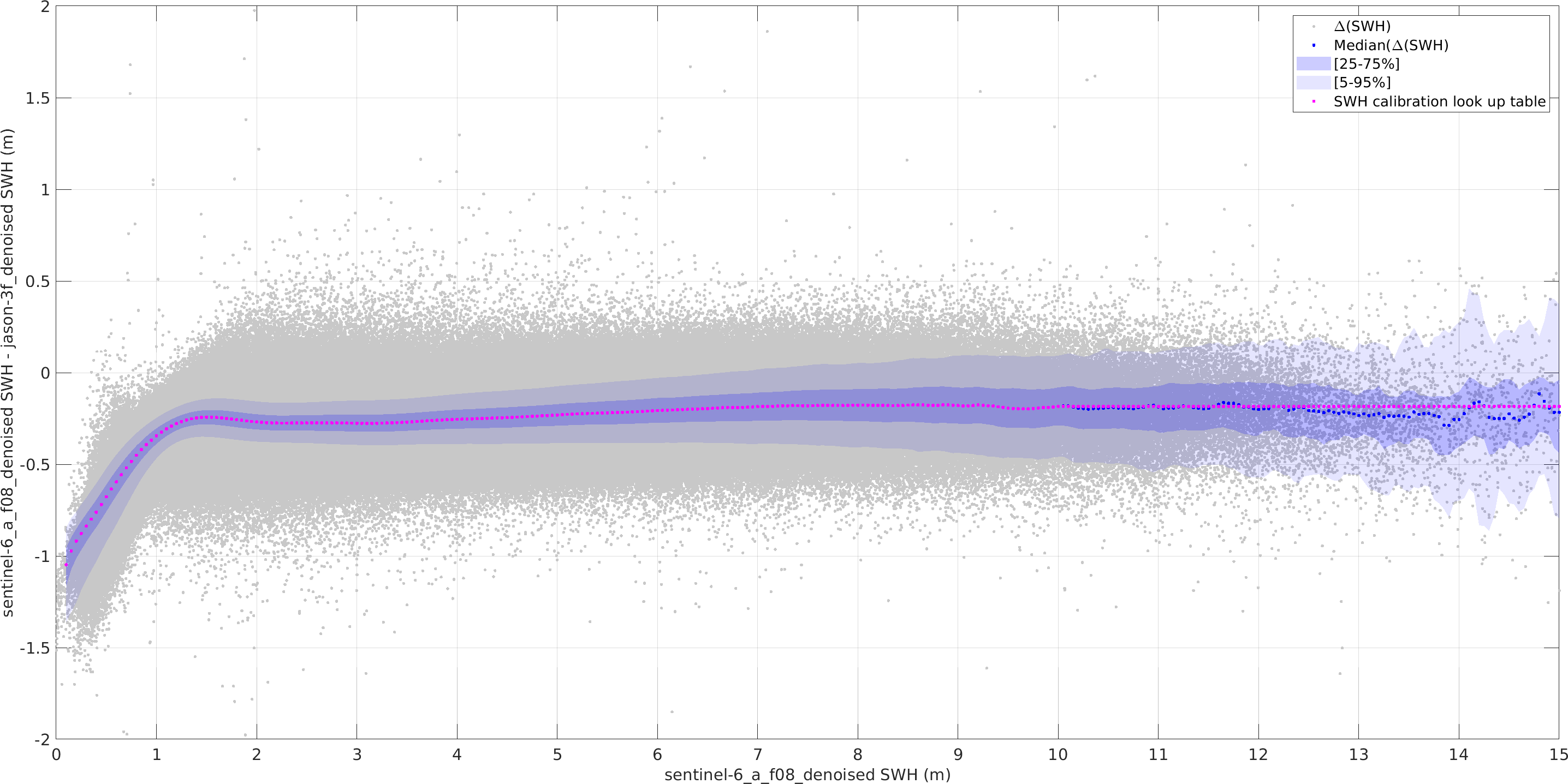
Fig. 4.5 Median of the differences between SWH (tandem) records from Sentinel-6A/MF and Jason-3 computed over SWH bins of 0.2m and shifted by 0.05m. Grey dots show each data pair differences (22,442,832 records), blue dots show the median value for each bin, ligh and dark shaded region indicate the [25-75%] and [5-95%] limits of the distribution for each bin, and magenta dots show the final Look Up Table after extrapolation of the correction above 10m.

However, for most of the non-tandem cases, the number of data pairs is generally too low between 5 to 10m so that the correction LUT contains NaN values or appear noisy overt this range. In such cases, a robust linear regression is fitted through the median of the residuals over a mission-specific SWH range (generally between 2 to 7m) to model the error function above a specific threshold. Fig. 4.6 provides such an example with the intercalibration between Sentinel-3A and Jason-3. These thresholds and ranges are estimated by visual inspection of the data in order to ensure an accurate representation of the bias structure and a smooth transition between the non-linear corrections for low-to-medium sea state conditions and the linear corrections for medium-to-high sea state conditions. Finally, a 5-point moving average is applied to the corrections in order to reduce small scale oscillations.

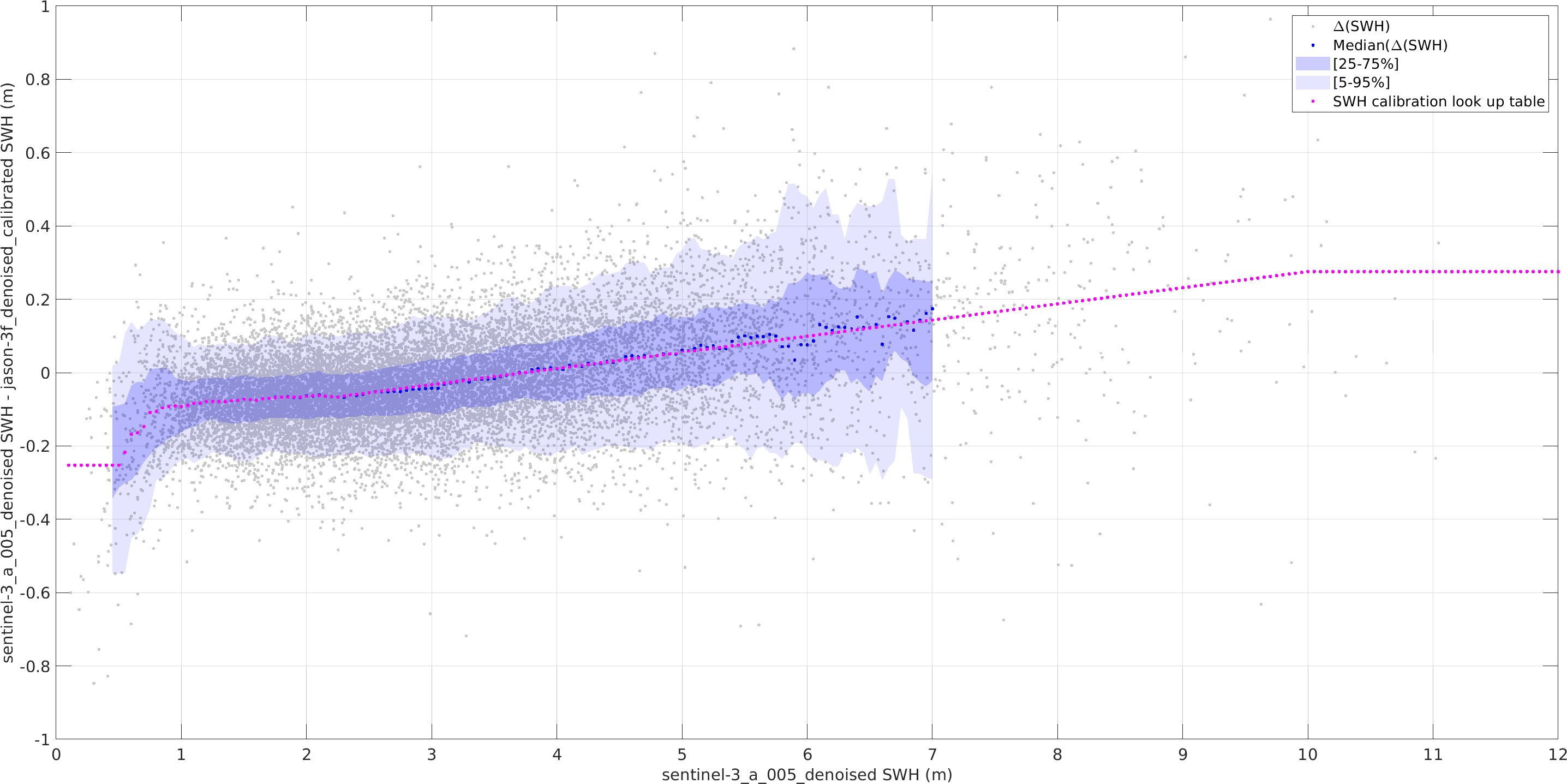
Fig. 4.6 Median of the differences between SWH (crossover) records from Sentinel-3A and Jason-3 computed over SWH bins of 0.2m and shifted by 0.05m. Grey dots show each data pair differences (14,224 records), blue dots show the median value for each bin, ligh and dark shaded region indicate the [25-75%] and [5-95%] limits of the distribution for each bin, and magenta dots show the final Look Up Table after extrapolation of the correction above 10m.

4.5.6.2. Selection of in situ platforms for absolute calibration

The CMEMS In Situ Thematic Assembly Center (CMEMS INSTAC) is a component of the European Marine Copernicus Service and its role is to ensure consistent and reliable access to a range of in situ data for service production and validation. For this purpose, CMEMS INSTAC collects multi-source/multiplatform data, and performs consistent quality control before distributing the data in a common format to the CMEMS Marine Forecasting Centres (MFC). The data can be found at http://www.marineinsitu.eu/. For the absolute calibration of the SWH records from the reference missions, we have considered all altimeter-in situ matchups for which the the altimeter records was located at a minimum distance of 50 km from the shore, a maximum distance of 50 from the buoy, and with a maximum time difference of 30min with the buoy records. In order to ensure that only good quality measurements are selected, a number of tests have been applied:

• stationarity: rejecting SWH buoy measurements having a constant SWH value over more than 48 hr;

• location: rejecting SWH buoy measurements over unrealistic position change within a short period of time;

• CMEMS quality check: using the CMEMS native quality flags on time, location and SWH to reject bad or suspect SWH buoy measurements;

• precision: detecting and rejecting SWH buoy measurements having a precision equal or larger than 0.5 meters;

• range: rejecting SWH buoy measurements out of the 0-30 meter range;

• Matchups between altimeter and in situ platform measurements were computed within 100-km distance and 1-h time window. The in situ SWH observations were smoothed with a 1-h running average, in order to reduce high-frequency variability.

Note

Note on the drift correction of TOPEX Side A SWH The TOPEX altimeter was the primary sensor for the TOPEX/POSEIDON mission. It is a redundant instrument, with the two sides designated Side A and Side B. The TOPEX Side A altimeter was activated soon after launch. It began to show signs of change/degradation in early 1997. In particular, changes in the Side A point target response were observed as an apparent drift in the measured significant wave heights and instrument range RMS, and as a result Side A was turned off on February 10, 1999 and Side B turned on, becoming the new primary operational altimeter (Rosmorduc et al., 2023). The TOPEX Side A and Side B SWH records are therefore considered as two separate dataset. In the CCI v4, we use the latest CNES/JPL reprocessing : TOPEX/POSEIDON GDR-F Products. As detailed in the product handbook (Rosmorduc et al. 2023), the TOPEX altimeter data processing used for this product is based upon a numerical retracking approach, which introduces the instrument Point Target Response (PTR) to obtain an echo model that better reflects the characteristics of the altimeter. Unlike the classical analytical MLE solution, no instrument corrections are needed with the numerical retracking approach for range, SWH and sigma0 as a function of SWH and off nadir angle (i.e., Look Up Tables are not required or applied). In addition, the use of the measured PTR compensates for the impact of the altimeter evolution on the range, SWH and sigma0 measurements without having to introduce external corrections. In particular, this approach allows for much more stable SWH measurements when compared to the original TOPEX dataset. Given the objective of long-term cross mission consistency of the CCI v4, intercalibration was deemed necessary and a LUT was also derived for this mission. However, since TOPEX Side A was turned off before the launch of the subsequent reference mission (Jason-1), its SWH intercalibration is based on crossover records with ERS-2. Time consistency of TOPEX Side A was assessed through comparisons with the Ifremer WW3 and ECMWF ERA-5 wave model hindcasts, which revealed a slightly decreasing trend of the SWH records over the period July 1994 to February 1999. This trend was linearly corrected using model results interpolated along the track.

References

Dodet, G., Piolle, J.-F., Quilfen, Y., Abdalla, S., Accensi, M., Ardhuin, F., Ash, E., Bidlot, J.-R., Gommenginger, C., Marechal, G., Passaro, M., Quartly, G., Stopa, J., Timmermans, B., Young, I., Cipollini, P., Donlon, C. , 2020. The Sea State CCI dataset v1: towards a sea state climate data record based on satellite observations. Earth System Science Data 12, 1929–1951. https://doi.org/10.5194/essd-12-1929-2020

Queffeulou, P., 2016. Validation of Jason-3 altimeter wave height measurements. Presented at the OSTST.

Rosmorduc, V., Roinard, H., Desai, S., Desjonqueres, J.-D., Callahan, P.S., Bignalet-Cazalet, F., 2023. TOPEX/POSEIDON GDR-F Products Handbook (No. SALP-MU-MAO-OP-17607-CN).

Sepulveda, H., Queffeulou, P., Ardhuin, F., 2015. Assessment of SARAL/AltiKa Wave Height Measurements Relative to Buoy, Jason-2, and Cryosat-2 Data.
Marine Geodesy 38, 449–465. https://doi.org/10.1080/01490419.2014.1000470

4.5.7. Denoising

A non-parametric denoising method based on Empirical Mode Decomposition (EMD, Huang et al., 1998) and inspired by wavelet thresholding is applied to the bias corrected variable swh_adjusted and stored in swh_denoised (see Kopsinis and McLaughlin, 2009, Quilfen et al., 2018 and Quilfen and Chapron, 2019ab).

A detailed description of the method can be found in Quilfen and Chapron, 2019b.

For a given noisy, input signal, the SNR and robustness of the denoised signal (e.g. to mitigate for result uncertainties associated with signal fluctuations close to the applied thresholds) are increased by estimating the final result as an ensemble average of several denoised signals. For that, the noise n1(t) is first removed from the noisy signal x(t), then a set of k new noisy signals is generated by adding random realisations of n1(t), providing after denoising a set of k denoised signals whose average gives the resulting denoised SWH swh_denoised and whose standard deviation gives the uncertainty attached to the denoised SWH (swh_emd_uncertainty). The uncertainty parameter swh_emd_uncertainty therefore accounts for the noise characteristics of the noisy signal (function of the altimeter sensor, SWH etc), as well as for the local SNR (which is scale-dependent) and for uncertainties attached to the denoising process.

References

Huang, N.E., Shen, Z., Long, S.R., Wu, M.C., Shih, H.H., Zheng, Q., Yen, N.-C., Tung, C.C., Liu, H.H., 1998. The empirical mode decomposition and the Hilbert spectrum for nonlinear and non-stationary time series analysis. Proceedings of the Royal Society of London A: Mathematical, Physical and Engineering Sciences 454, 903–995. https://doi.org/10.1098/rspa.1998.0193

Kopsinis, Y., McLaughlin, S., 2009. Development of EMD-Based Denoising Methods Inspired by Wavelet Thresholding. IEEE Transactions on Signal Processing 57, 1351–1362. https://doi.org/10.1109/TSP.2009.2013885

Quilfen, Y., Yurovskaya, M., Chapron, B., Ardhuin, F., 2018. Storm waves focusing and steepening in the Agulhas current: Satellite observations and modeling. Remote Sensing Of Environment 216, 561–571. https://doi.org/10.1016/j.rse.2018.07.020

Quilfen, Y., and Chapron, B., 2019. Ocean Surface Wave-Current Signatures From Satellite Altimeter Measurements. Geophysical Research Letters 46, 253–261. https://doi.org/10.1029/2018GL081029

Quilfen Y., Chapron B. (2020). On denoising satellite altimeter measurements for high-resolution geophysical signal analysis. Advances in Space Research, 68. https://doi.org/10.1016/j.asr.2020.01.005]

4.5.8. Uncertainties

The L2P files contain two different and complementary estimates of uncertainty:

• swh_emd_uncertainty: this is based on the “noise” estimated from the along-track variability of the EMD denoising applied on the 1 Hz data. It is an estimate of the uncertainty of the debiased and denoised significant wave height.

• swh_uncertainty: this is a theoretical estimate of the uncertainty caused by speckle noise and sampling in 1-Hz averaged SWH values. Note that SWH sampling errors at 1Hz can be correlated (e.g. De Carlo et al. 2023), so that the average over n 1~Hz values can have an uncertainty larger than 1/sqrt(n) times the 1 Hz uncertainty.

For the largest wave heights (Hs > 15 m) we advise to make a distinction between Hs and SWH: SWH is an average of local wave heights, and it contains fluctuations due to sampling uncertainty (i.e. wave groups), and the true significant wave height Hs can only be estimated by averaging or denoising. We find that the uncertainty on Hs estimated from a 7-point running average and applying the theoretical uncertainty model for 7 s averages is close to the EMD denoising uncertainty estimate.

The theoretical uncertainty is fully described in De Carlo and Ardhuin (2024), and the variance is the sum of a variance caused by speckle noise and sampling (wave group effect).

For speckle noise, it is a function of the wave height Hs, the number of pulses averaged \(n_a\), and the retracking method: Maximum Likelihood (ML), WHALES or Least Squares (LS), and a variance caused by sampling (wave group effect) which is a function of the wave height Hs, the satellite altitude h and the spectral shape quantified by the peakedness \(Q_{kk}\)).

The processing algorithm sets the value of s0 which gives the effect of speckle noise: it is lowest for ML (s0=1 m), intermediate for WHALES (s0 ~ 2 m) and largest for LS (s0=5 m).

The all_sat_uncertainties shows estimated of (a) the effective spatial resolution of the along-track altimeter data: this is roughly the Chelton et al. (1989) radius \(\rho_c\)=sqrt(2 h Hs) divided by 1.5, this is smallest for CFOSAT because of the much lower orbit (b) the uncertainty of the data at the native rate (4.5 Hz for CFOSAT, 40 Hz for SARAL and 20 Hz for all others) and (c) the uncertainty of SWH averaged over 1 Hz. Note that there was a mistake in a similar figure of De Carlo and Ardhuin (2024) for CFOSAT (the native data rate was not properly taken to be 4.5 Hz)

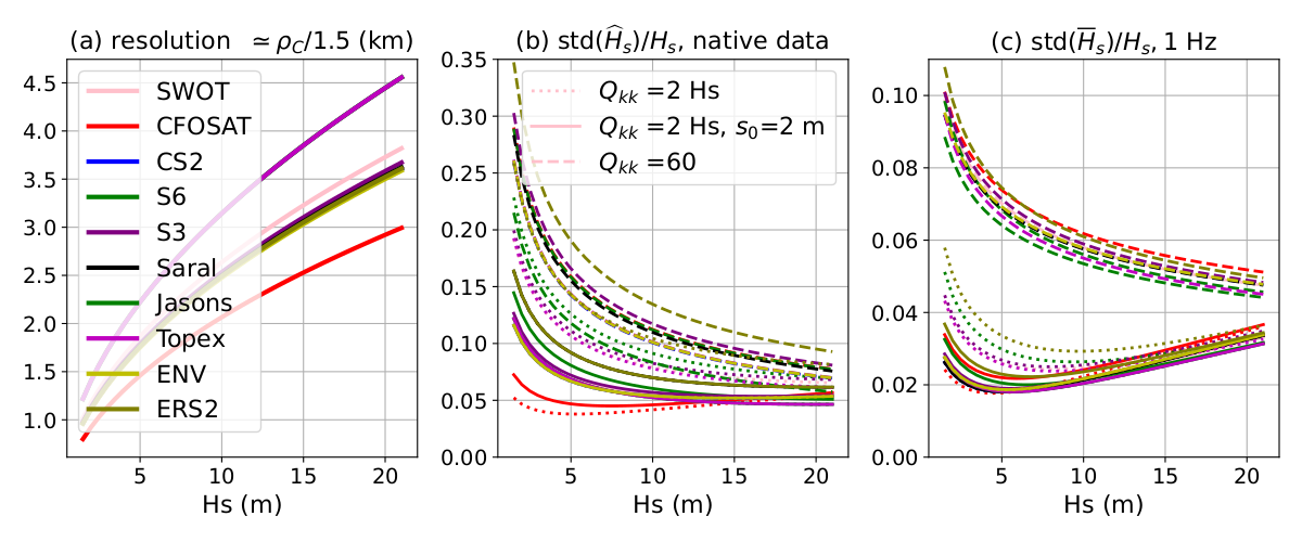
Different spectral shapes are considered: \(Q_{kk}\) = 2 Hs is typical of a wind sea, whereas swell-dominated conditions often have \(Q_{kk}\) > 60 m.